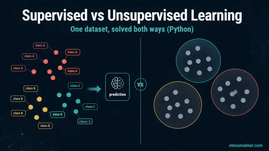
Quick answer: The difference between supervised and unsupervised learning is the labels. In supervised learning, every training example comes with the correct answer (a label), and the model learns to predict that answer for new data, as in “spam or not spam”. In unsupervised learning, there are no labels, and the model looks for structure on its own, such as groups of similar customers. Use supervised learning when you know what you want to predict and have labeled examples. Use unsupervised learning when you want to explore data or have no labels.
This guide takes one real dataset and solves it both ways in Python, so you can see what each approach gives you, how each one is checked, and a common scaling mistake that can wreck clustering results without any error. All the code runs in a few seconds with scikit-learn and needs no downloads.
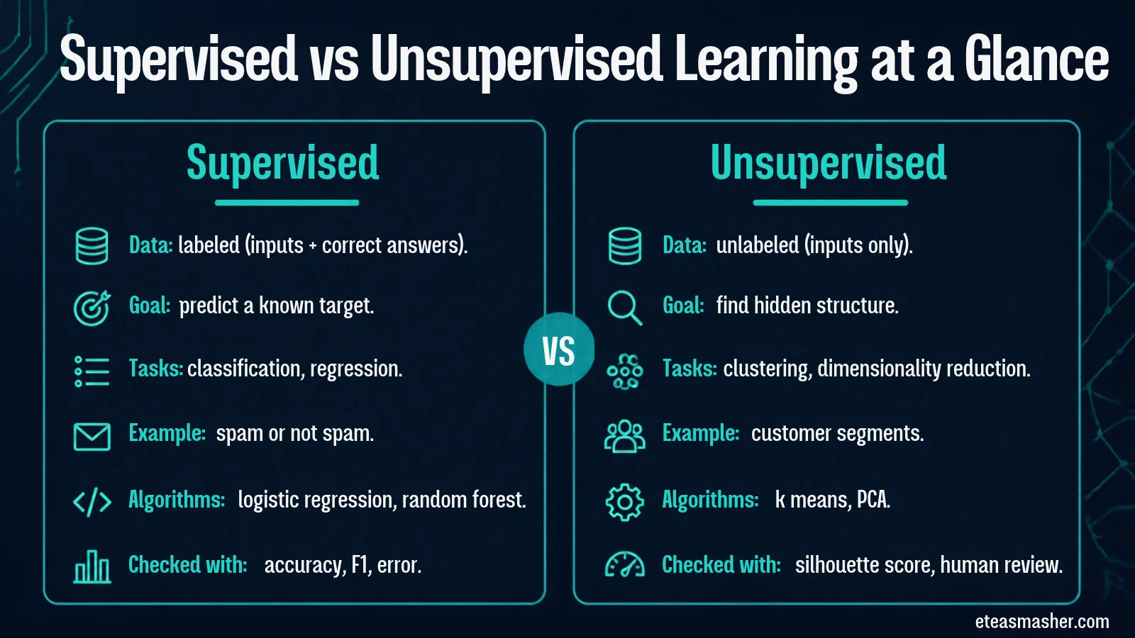
Linear and logistic regression, decision trees, random forest, gradient boosting
k-means, hierarchical clustering, DBSCAN, PCA
How you check it
Compare predictions with held-out true labels (accuracy, F1, error)
Internal scores (such as silhouette) plus human judgment
Main cost
Getting enough correct labels
Results can be hard to interpret or verify
Supervised learning predicts a known target; unsupervised learning finds structure without labels.
What is supervised learning?
Supervised learning trains a model on examples where the correct answer is already known. The model sees the inputs (features) and the matching outputs (labels), and adjusts itself to reduce its errors on those labels. Once trained, it predicts labels for data it has never seen.
It comes in two forms:
Classification predicts a category: spam or not spam, which disease, which grape variety.
Regression predicts a number: a house price, tomorrow’s temperature, next month’s sales.
A common source of confusion: logistic regression is a classification method, despite its name. It predicts the probability of each class and picks the most likely one.
Someone has to create the labels. For emails, users label spam for free when they click “report spam”. For medical images, a trained doctor may need to label every scan, which is slow and expensive. Label cost is often what decides whether supervised learning is practical.
What is unsupervised learning?
Unsupervised learning works with inputs only. There is no correct answer to learn from, so the algorithm looks for patterns in how the data points relate to each other.
The main tasks are:
Clustering puts similar data points into groups, for example customer segments based on buying habits.
Dimensionality reduction compresses many features into fewer ones while keeping as much of the variation in the data as possible, which helps with visualization and speeds up later models. PCA is the classic method.
Anomaly detection flags points that don’t fit any normal pattern, such as an unusual bank transaction.
Checking the result is harder. Without labels, there is no simple score that says the clusters are “right”. You judge them with internal measures and, above all, by whether the groups make sense to someone who knows the domain.
One dataset, solved both ways
To compare the two approaches fairly, we will use the same data for both: the wine dataset that comes with scikit-learn. It contains 178 wines, each described by 13 chemical measurements (alcohol, magnesium, color intensity and so on), from 3 grape varieties grown in the same region of Italy. It originally comes from the UCI Machine Learning Repository.
The labels (the grape variety of each wine) are what make this a good test. In the supervised version we give them to the model. In the unsupervised version we hide them, and only use them at the very end to check how close the clusters came.
You only need scikit-learn and pandas (pip install scikit-learn pandas).
Step 1: Load the data
import pandas as pd
from sklearn.datasets import load_wine

X, y = load_wine(return_X_y=True, as_frame=True)
print(X.shape)                                  # 178 wines, 13 measurements
print(y.value_counts().sort_index().to_dict())  # wines per grape variety
(178, 13)
{0: 59, 1: 71, 2: 48}
Step 2: The supervised way (labels given)
Here the question is: given a wine’s chemistry, which grape variety is it? We train a logistic regression classifier on 75% of the wines and test it on the 25% it has never seen.
Two tools in the code are worth knowing. StandardScaler rescales each feature to a mean of 0 and a standard deviation of 1, so features measured in big units don’t outweigh small ones. make_pipeline chains the scaler and the model, so the scaler is fitted only on training data each time. That avoids a quiet form of data leakage, where information from the test set slips into training.
from sklearn.model_selection import train_test_split, cross_val_score
from sklearn.pipeline import make_pipeline
from sklearn.preprocessing import StandardScaler
from sklearn.linear_model import LogisticRegression
from sklearn.metrics import accuracy_score

# stratify=y keeps the same mix of varieties in both sets; random_state makes it repeatable
X_train, X_test, y_train, y_test = train_test_split(
    X, y, test_size=0.25, random_state=42, stratify=y)

# Scale the features, then classify. max_iter gives the solver enough steps to finish.
clf = make_pipeline(StandardScaler(), LogisticRegression(max_iter=1000))
clf.fit(X_train, y_train)
print("Test accuracy:", round(accuracy_score(y_test, clf.predict(X_test)), 3))

# A 45-wine test set is small, so check with 5-fold cross-validation too
scores = cross_val_score(clf, X, y, cv=5)
print("5-fold accuracy:", round(scores.mean(), 3), "+/-", round(scores.std(), 3))
Test accuracy: 1.0
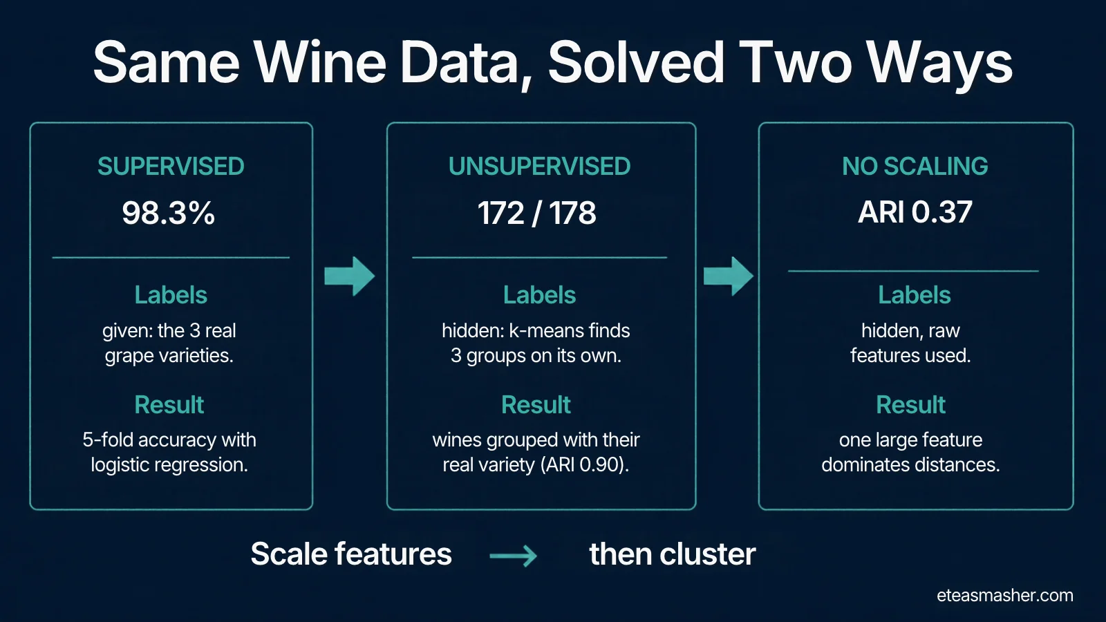
5-fold accuracy: 0.983 +/- 0.014
The model got every one of the 45 test wines right. That sounds perfect, but a test set of 45 is small, and one lucky split can flatter a model. Cross-validation trains and tests five times on different splits and gives a more honest figure: 98.3% average accuracy. The “+/- 0.014” is the standard deviation across the five runs; the individual folds scored between 97.1% and 100%. Supervised learning is easy to evaluate because we have the right answers to compare against.
Step 3: The unsupervised way (labels hidden)
Now we pretend nobody ever told us the grape varieties. The question becomes: are there natural groups of wines in this chemistry data, and how many?
We use k-means clustering, which splits the data into k groups so that each wine is as close as possible to the center (average point) of its group. But k-means needs us to choose k. Without labels, a common way to choose is the silhouette score, which measures how well each point fits its own cluster compared with the nearest other cluster. It runs from -1 to 1: higher is better, values near 0 mean the groups overlap, and negative values suggest points sit in the wrong cluster.
from sklearn.cluster import KMeans
from sklearn.metrics import silhouette_score

X_scaled = StandardScaler().fit_transform(X)

for k in range(2, 7):
    # n_init=10 runs k-means 10 times from different starting points and keeps the best
    km = KMeans(n_clusters=k, n_init=10, random_state=42).fit(X_scaled)
    print(f"k={k}  silhouette={silhouette_score(X_scaled, km.labels_):.3f}")
The score is highest at k = 3, but only slightly (0.285 against about 0.26 for k = 2 and k = 4), and all the scores are low, which means the groups overlap quite a bit. So k = 3 is a reasonable choice, not proof. Here it happens to match the three grape varieties; in a real project you would not know that.
Now we cluster with k = 3 and, for the first time, compare the clusters with the hidden labels. Cluster numbers are arbitrary (k-means might call a group “0” or “2”), so we can’t compare them with the varieties directly. Instead we use the adjusted Rand index (ARI), which compares two groupings regardless of their names. It is 1 for a perfect match and around 0 for random grouping (it can dip slightly below 0).
from sklearn.metrics import adjusted_rand_score

km = KMeans(n_clusters=3, n_init=10, random_state=42).fit(X_scaled)

# Labels are used ONLY now, to check how close the clusters came
print("ARI:", round(adjusted_rand_score(y, km.labels_), 3))
print(pd.crosstab(y, km.labels_, rownames=["real variety"], colnames=["cluster"]))
The table shows that each cluster lines up with one grape variety. All 59 wines of variety 0 landed in cluster 2, all 48 of variety 2 landed in cluster 1, and 65 of the 71 wines of variety 1 landed in cluster 0. That is 172 of 178 wines grouped with their real variety, and an ARI of 0.897, without the model ever being told the varieties existed.
Step 4: The scaling trap
Both versions above scaled the features first with StandardScaler. Here is what happens to the clustering without it:
km_raw = KMeans(n_clusters=3, n_init=10, random_state=42).fit(X)   # raw, unscaled
print("ARI without scaling:", round(adjusted_rand_score(y, km_raw.labels_), 3))

# What would the silhouette score have told us?
print("Silhouette, unscaled:", round(silhouette_score(X, km_raw.labels_), 3))
print("Silhouette, scaled:  ", round(silhouette_score(X_scaled, km.labels_), 3))
ARI without scaling: 0.371
Silhouette, unscaled: 0.571
Silhouette, scaled:   0.285
The match with the real varieties drops from 0.897 to 0.371. The reason is in the units. One feature, proline, ranges from 278 to 1,680, while hue ranges from 0.48 to 1.71. K-means measures plain distances, so a difference of 100 in proline outweighs everything that happens in hue. In fact, running k-means on proline alone gives exactly the same three groups as the unscaled run: the other 12 measurements play no part at all.
Now look at the silhouette scores. The unscaled clustering scores 0.571, twice the scaled version’s 0.285. The very tool we used to choose k says the bad clustering is better. The silhouette score is measured in whatever feature space you give it, so it cannot tell you whether your scaling choice was right.
That is the practical lesson of this comparison: distance-based unsupervised methods such as k-means are very sensitive to feature scale, and the usual checks can point the wrong way. The code runs, you get three clusters, and the internal score even looks good. In the supervised version, the same mistake at least leaves traces: without scaling, logistic regression drops to about 96% cross-validated accuracy, and scikit-learn warns that the model did not converge.
Results from the code in this article: scaling decides whether clustering works.
What the experiment shows
Supervised (logistic regression)
Unsupervised (k-means)
Question asked
Which variety is this wine?
What groups exist in this data?
Used the labels?
Yes, for training
No (only for our final check)
Result
98.3% cross-validated accuracy
172 of 178 wines grouped with their real variety, ARI 0.90
How we knew it worked
Compared with known answers
Silhouette score to pick k; labels only because this is a demo
What can quietly go wrong
Too-small test set or data leakage gives a flattering score
Unscaled features drop ARI from 0.90 to 0.37 while the silhouette score rises
Two things to take away:
Supervised learning gives you a clear report card, as long as your test data is honest. Unsupervised learning does not. In a real clustering project you would have no hidden labels to check against. You would rely on the silhouette score, on looking at what each cluster contains, and on whether people who know the domain find the groups useful.
The two approaches work well together. A common pattern is to explore with unsupervised methods first (to find segments or spot outliers), then label some data and train a supervised model for the prediction you actually need.
How to choose between them
Ask these questions in order:
Do you have a specific thing you want to predict? If yes, you are heading toward supervised learning. If you just want to understand or organize the data, start with unsupervised learning.
Do you have labels for it, or can you get them at a reasonable cost? If yes, use supervised learning. If labels are rare or expensive, consider semi-supervised learning (below) or start unsupervised.
How will you know if it worked? Supervised projects can be scored against held-out labels. For unsupervised projects, decide upfront how you will judge the result, for example by asking whether a marketing team can act on the customer segments.
Situation
Better fit
Predict which customers will cancel, with past cancellation records
Supervised (classification)
Estimate house prices from past sales
Supervised (regression)
Split customers into segments for different campaigns
Unsupervised (clustering)
Spot unusual transactions when fraud is rarely labeled
Unsupervised (anomaly detection), often followed by human review
Reduce 200 features to a few for a chart or a faster model
Unsupervised (dimensionality reduction)
Beyond the two: semi-supervised, self-supervised and reinforcement learning
Supervised and unsupervised learning are the two classic types, but three related approaches come up often.
Semi-supervised learning uses a small labeled set plus a large unlabeled one. For example, an online shop might hand-tag 500 support tickets by topic and let the model also learn from 50,000 untagged ones. It is useful when labels are expensive.
Self-supervised learning creates labels automatically from the data itself. Large language models are pretrained this way: the label for each position in a text is the next token (a word or part of a word), so no human has to label that stage. Later training stages do use human-written examples and feedback. Our guide on how large language models work explains this training step in detail.
Reinforcement learning learns by trial and error from rewards, rather than from labeled examples, for example a program learning to play a game by being rewarded for winning.
Common mistakes
Forgetting to scale before clustering. In our example it dropped the ARI from 0.90 to 0.37 with no error message, and the silhouette score got better, not worse.
Trusting a single small test split. Use cross-validation, as we did, before believing a near-perfect score.
Treating cluster numbers as meaningful. Cluster “0” is just a name. Read what is inside each cluster before giving it a business label.
Using features you won’t have at prediction time. If a feature is only known after the event you are predicting (such as “refund issued” when predicting complaints), the model will look great in testing and fail in real use. This is called data leakage. Fitting a scaler on all the data before splitting is a smaller version of the same problem, which is why the example uses a pipeline.
Frequently asked questions
What is the main difference between supervised and unsupervised learning?
Supervised learning trains on labeled data, meaning each example includes the correct answer, and learns to predict that answer for new data. Unsupervised learning trains on unlabeled data and finds structure, such as groups or patterns, on its own.
Is clustering supervised or unsupervised?
Clustering is unsupervised. Algorithms such as k-means group data points by similarity without using any labels. If you already know the categories and want to assign new items to them, that is classification, which is supervised.
Is regression supervised or unsupervised?
Regression is supervised. It learns from examples with known numeric outcomes, such as past house prices, to predict the number for new examples.
Which is better, supervised or unsupervised learning?
They answer different questions. Supervised learning is the right tool when you need to predict a known target and have labels. Unsupervised learning is the right tool for exploring data, finding segments or spotting anomalies when labels don’t exist.
Do I need to scale my data for unsupervised learning?
For distance-based methods such as k-means, yes, unless all your features are already in the same units. In our wine example, skipping scaling dropped the match with the real grape varieties from an ARI of 0.90 to 0.37, because one feature with large values decided the clusters on its own.
Key points
Supervised learning learns from labeled examples to predict a known target; unsupervised learning finds structure in unlabeled data.
On the same wine data, supervised logistic regression reached 98.3% cross-validated accuracy, and unsupervised k-means grouped 172 of 178 wines with their real variety without seeing any labels.
Supervised results are easy to check against known answers; unsupervised results need internal scores and human judgment.
Scale your features before distance-based clustering, and don’t rely on the silhouette score to catch a scaling mistake.